
I work in IT. As a function of my job, I know a lot of little tips and tricks for many programs. Excel is one of my go-to programs, but I rarely use it for numbers – I generate code and do a lot of data work with it instead.
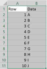
I recently had a long list of information to print out as reference material. It contained several columns, and I wanted a quick way to follow the information across the printed row without having to use an external guide.
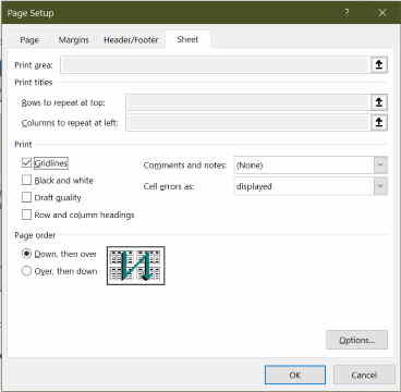
I could have used “print gridlines” to put the grid lines on, but this only marginally improve readability.
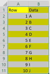
I decided to color every other row in the selection a light grey. I could have done this by hand-formatting the rows, but I had thousands of lines to do. Here is what I did to highlight the cells using conditional formatting:
Highlighting Rows With Conditional Formatting
- Select all the cells you wish to change.
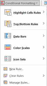
- Choose Conditional Formatting from the Home ribbon and choose New Rule.
- Select “use a formula” from the Rule Type.
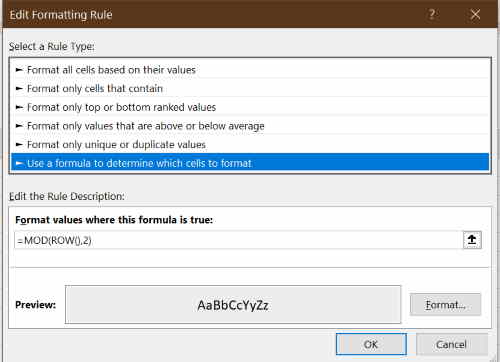
- Enter “=MOD(ROW(),2)” in the formula box.
- Select the formatting by pressing on the format button.
- Click OK.
And you now have highlighted rows.


3 Comments
LJ
One of my excellent readers, Filipe from Brazil, pointed out the formula is “=mod(lin(),2)” for those people using the Portuguese version of Excel.
Robert Parker
Very cool. Works well and saves a lot of time. Thanks for this tip.
Ronan Allen
Very Useful